グラフ
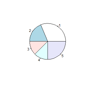
円グラフ (pie chart)
pie(
    x,
    labels = names(x),
    edges = 200,
    radius = 0.8,
    clockwise = FALSE,
    init.angle = if(clockwise) 90 else 0,
    density = NULL,
    angle = 45,
    col = NULL,
    border = NULL,
    lty = NULL,
    main = NULL,
    ...)
R: Pie Charts
a <- c(50,30,20,20,40)
pie(a)
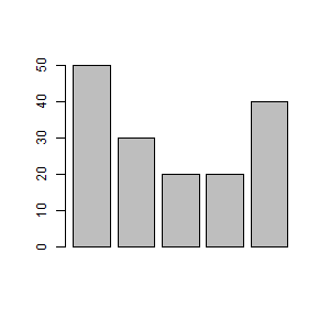
棒グラフ (bar chart)
barplot(
    height,
    ...)
R: Bar Plots
a <- c(50,30,20,20,40)
barplot(a)
箱型図 (box plot)
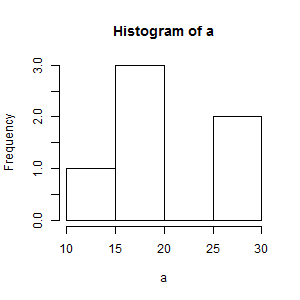
ヒストグラム (histogram / 柱状図)
hist(x, ...)R: Histograms
a <- c(30,30,10,20,20,20)
hist(a)
引数のxは、数値 (NumericまたはInteger) でなければなりません。もし次のようにそれ以外の型を渡すならば、数値部分だけを渡すようにします。
> (a <- read.table("sample.txt"))
  V1
1 10
2 20

> hist(a)
 hist.default(a) でエラー:  'x' は数値でなければなりません

> hist(a$V1)
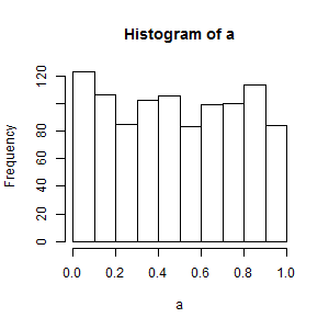
階級幅
既定ではbreaks="Sturges"が適用され、その値はnclass.Sturges()により求められます。
nclass.Sturges(x)R: Compute the Number of Classes for a Histogram
> a <- runif(1000)

> nclass.Sturges(a)
[1] 11

> hist(a)
> hist(a,breaks=100)
| 既定値 (breaks="Sturges") | breaks=100 |
|---|---|
 |
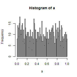 |
折れ線グラフ (ine graph)
散布図 (scatterplot)
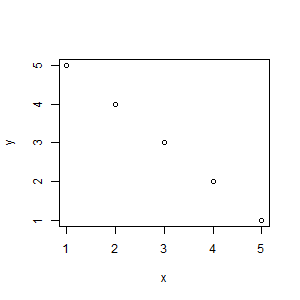
plot(x, y, ...)R: Generic X-Y Plotting
x <- c(1,2,3,4,5)
y <- c(5,4,3,2,1)
plot(x,y)
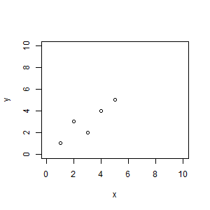
x軸とy軸の範囲は、xlimとylimで指定できます。
a <- data.frame(x=c(1,3,2,4,5), y=1:5)
plot(a, xlim=c(0,10), ylim=c(0,10))
付随処理
点の描画
points(x, ...)R: Add Points to a Plot
plot(NULL, xlim=c(0,5), ylim=c(0,5))

points(1, 1)
points(2, 2, col=2) # 色を指定
points(3, 1, cex=3) # 大きさを指定
points(4, 2, pch=8) # 形状を指定
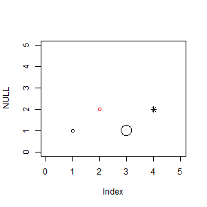
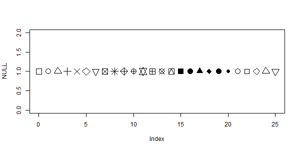
描画する記号は、pchの値によって変更できます。
plot(NULL, xlim=c(0,25), ylim=c(0,2))
points(data.frame(x=0:25, y=1), pch=0:25, cex=2)
ファイルへの出力
コマンドで出力
png(file="sample.png", width=300, height=300) # ファイルを生成
pie(data) # グラフを描画
dev.off() # デバイスを閉じ、ファイルへ出力
R Graphicsから出力
R Consoleからグラフを出力すると表示されるR GraphicsのGUIで、メニューの【ファイル → 別名で保存】からファイルへ出力できます。