統計解析
集計
> (a <- read.table("sample.txt"))
  V1  V2
1  1  40
2  1  60
3  2 120
4  2  80
5  1  50


> (g <- group_by(a, V1))          # V1列で分類
Source: local data frame [5 x 2]
Groups: V1 [2]

     V1    V2
  <int> <int>
1     1    40
2     1    60
3     2   120
4     2    80
5     1    50


> summarise(g, sum(V2), mean(V2)) # 分類した結果に対して、V2列の合計と平均を出力
# A tibble: 2 × 3
     V1 `sum(V2)` `mean(V2)`
  <int>     <int>      <dbl>
1     1       150         50
2     2       200        100
group_by(.data, ..., add = FALSE)R: Group a tbl by one or more variables.
summarise(.data, ...)R: Summarise multiple values to a single value.
統計
分散
分散 (実際は標本分散) と、共分散または相関を求められます。
var
var(x,
  y = NULL,
  na.rm = FALSE,
  use)
> var(1:10)
[1] 9.166667
cor
cor(
  x,
  y = NULL,
  use = "everything",
  method = c("pearson", "kendall", "spearman"))
R: Correlation, Variance and Covariance (Matrices)
標準偏差
標準偏差 (実際は標本標準偏差) を求められます。
sd(
  x,
  na.rm = FALSE)
R: Standard Deviation
> sd(1:10)
[1] 3.02765
クラスタリング
階層的クラスタリング (Hierarchical Clustering)
hclust(
    d,
    method = "complete",
    members = NULL)
R: Hierarchical Clustering
k平均クラスタリング (K-Means Clustering) / k平均法
kmeans(
    x,
    centers,
    iter.max = 10,
    nstart = 1,
    algorithm = c(
        "Hartigan-Wong",
        "Lloyd",
        "Forgy",
        "MacQueen"),
    trace=FALSE)
R: K-Means Clustering
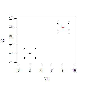
> (a <- read.table("sample.txt")) # 対象データを読み込み
  V1 V2
1  3  1
2  1  3
3  3  3
4  7  7
5  9  7
6  7  9
7  9  9
8  1  1

> plot(a, xlim=c(0,10), ylim=c(0,10)) # 対象データを描画


> (cl <- kmeans(a, 2)) # クラスタリングを実行
K-means clustering with 2 clusters of sizes 4, 4

Cluster means:
  V1 V2
1  8  8
2  2  2

Clustering vector:
[1] 2 2 2 1 1 1 1 2

Within cluster sum of squares by cluster:
[1] 8 8
 (between_SS / total_SS =  90.0 %)

Available components:

[1] "cluster"      "centers"      "totss"
[4] "withinss"     "tot.withinss" "betweenss"
[7] "size"         "iter"         "ifault"

> points(cl$centers, col=1:2, pch=19) # クラスター中心を描画
> cbind(a,cl$cluster) # 要素にクラスター番号を併記して確認
  V1 V2 cl$cluster
1  3  1          2
2  1  3          2
3  3  3          2
4  7  7          1
5  9  7          1
6  7  9          1
7  9  9          1
8  1  1          2

> cbind(a,cl$cluster)[order(a[,"V1"]),] # "V1"列で並べ替えて確認
  V1 V2 cl$cluster
2  1  3          2
8  1  1          2
1  3  1          2
3  3  3          2
4  7  7          1
6  7  9          1
5  9  7          1
7  9  9          1

> a[order(cl$cluster),] # 要素をクラスター番号順に並べ替えて確認
  V1 V2
4  7  7
5  9  7
6  7  9
7  9  9
1  3  1
2  1  3
3  3  3
8  1  1
> a[cl$cluster==1,] #クラスター番号1に分類されている要素
  V1 V2
4  7  7
5  9  7
6  7  9
7  9  9

> a[cl$cluster==2,] #クラスター番号2に分類されている要素
  V1 V2
1  3  1
2  1  3
3  3  3
8  1  1
kmeansの成分
kmeans()が返すkmeansクラスのオブジェクトは、下表の成分を持ちます。
| 成分 | 値 |
|---|---|
| cl$cluster | [1] 1 1 1 2 2 2 2 1 |
| cl$centers |
V1 V2 1 2 2 2 8 8 |
| cl$totss | [1] 160 |
| cl$withinss | [1] 8 8 |
| cl$tot.withinss | [1] 16 |
| cl$betweenss | [1] 144 |
| cl$size | [1] 4 4 |
| cl$iter | [1] 1 |
| cl$ifault | [1] 0 |